10 Wrangle Data
10.1 A Data Wrangling Strategy
Data free of problems and ready for analysis rarely falls into our laptops. Data wrangling is the process of fixing problems that otherwise roadblock our analysis and adding features that unlock the potential of our data. As data analysts and researchers, there’s a sense of satisfaction that comes from overcoming these challenges. Performing this work in a script file, instead of changing the raw data file directly, preserves raw data in its original state and reproduces the analysis simply by executing code. Making our analyses reproducible enables our future selves and others to verify that they were performed correctly.
Common data problems include using an unconventional missing values coding scheme, impossible or erroneous values, messy and problematic data formats, cryptic, inaccurate, or problematic variable names, missing features, and categorical variables that are coded with numbers instead of explicit values like “female” and “male.”
Rarely do we write a script that solves all problems perfectly the first time. We often return to earlier sections to add code we did not initially realize was necessary. However, jumping around within a script can introduce sequence errors, where code written near the top relies upon code written lower down. These sequence errors can go initially undetected if the author executes the code as they write it. However, sequence errors will manifest when the author returns to a new session and executes code top-to-bottom or when the author renders the code. During rendering, R begins with an empty environment (no variables, data, or other objects in cache memory) and executes code line-by-line in the order of appearance. Sequence problems will now create errors.
An efficient and reliable data wrangling strategy is to fix problems immediately after import using a “recipe” of problem-solving commands linked together by either the base R, |>, or magrittr package, “%>%”, pipe operator. These two pipe operators function almost identically. Their subtle differences are not important for this lesson. The recipe is built progressively, adding and testing one component at a time. When complete, we have code that simultaneously imports data and fixes problems to produce a “mature” tibble ready for analysis, visualization, and statistics.
Starting an R script with “library(tidyverse)” is almost standard practice. The commands they provide are used in nearly every analysis. tidyverse is a collection of packages used to create and manipulate tidy data. For example, the tidyr package provides the pivot_longer and pivot_wider commands used to solve data format problems. The dplyr package provides commands like mutate, select and filter that add features or reduce a data set to features and observations of interest. The tidyverse authors maintain handy guides called vignettes that include fully reproducible examples, and downloadable cheat sheets. Links to those resources for tidyr and dplyr are here: tidyr vignette, tidyr Cheat Sheet, dplyr vignette, dplyr Cheat Sheet .
10.2 Inspect the data
Some problems can be identified after importing the data by viewing the data in tabular form and sorting the data by individual columns to view the smallest and largest values. Also useful, is to viewing the first few rows or “head” of the data and a summary of each column. The commands below develop familiarity with the data, such as by revealing variable types, missing values, and summary statistics.
Code
rm(list = ls())

# Import, summarize, and preview data
tbl <- read_csv('data/cholesterol.csv')
# View(tbl) # create a tabular data view, sort-able by individual columns. Do NOT include in script!
head(tbl) # show the first 6 rows of the data
# A tibble: 6 × 11
name age gender height group weight_i hdl_i ldl_i weight_f hdl_f ldl_f
<chr> <dbl> <dbl> <dbl> <dbl> <chr> <chr> <chr> <chr> <chr> <chr>
1 William 26 0 69 0 172 49 81 156 48 86
2 Richard 37 0 67 0 184 54 95 165 53 93
3 Joseph 45 0 66 0 191 49 106 180 46 112
4 Daniel 35 999 72 0 181 50 98 missing 51 100
5 Jennifer 44 1 64 0 203 44 107 189 47 111
6 Barbara 23 1 61 0 193 ### 103 187 59 111 Code
glimpse(tbl) # list the variables vertically, along with variable types and valuesRows: 40
Columns: 11
$ name <chr> "William", "Richard", "Joseph", "Daniel", "Jennifer", "Barbar…
$ age <dbl> 26, 37, 45, 35, 44, 23, 31, 44, 35, 41, 40, 33, 40, 54, 48, 2…
$ gender <dbl> 0, 0, 0, 999, 1, 1, 1, 1, 1, 1, 0, 0, 0, 0, 999, 1, 1, 1, 1, …
$ height <dbl> 69, 67, 66, 72, 64, 61, 61, 66, 62, 61, 63, 65, 69, 71, 58, 6…
$ group <dbl> 0, 0, 0, 0, 0, 0, 0, 0, 0, 0, 0, 0, 0, 0, 0, 0, 0, 0, 0, 0, 1…
$ weight_i <chr> "172", "184", "191", "181", "203", "193", "N/A", "192", "200"…
$ hdl_i <chr> "49", "54", "49", "50", "44", "###", "62", "54", "54", "48", …
$ ldl_i <chr> "81", "95", "106", "98", "107", "103", "107", "91", "98", "96…
$ weight_f <chr> "156", "165", "180", "missing", "189", "187", "177", "181", "…
$ hdl_f <chr> "48", "53", "46", "51", "47", "59", "60", "60", "###", "49", …
$ ldl_f <chr> "86", "93", "112", "100", "111", "111", "112", "101", "96", "…Code
summary(tbl) # Show summary statistics and the number of NA values for each variable name age gender height
Length:40 Min. :21.00 Min. : 0.0 Min. :54.00
Class :character 1st Qu.:32.50 1st Qu.: 0.0 1st Qu.:61.75
Mode :character Median :40.50 Median : 1.0 Median :65.00
Mean :39.62 Mean : 75.4 Mean :64.65
3rd Qu.:47.25 3rd Qu.: 1.0 3rd Qu.:67.00
Max. :55.00 Max. :999.0 Max. :74.00
group weight_i hdl_i ldl_i
Min. :0.0 Length:40 Length:40 Length:40
1st Qu.:0.0 Class :character Class :character Class :character
Median :0.5 Mode :character Mode :character Mode :character
Mean :0.5
3rd Qu.:1.0
Max. :1.0
weight_f hdl_f ldl_f
Length:40 Length:40 Length:40
Class :character Class :character Class :character
Mode :character Mode :character Mode :character
10.3 Code Missing Values
From the summary and head of the data created above, we can see that missing values are variably coded as 999 in the gender column, ### in the hdl_i column, and “missing” in the weight_f column. Also, something fishy is happening in the weight_i column. The tibble head shows numeric values, but the tbl summary indicates a character variable. By sorting the tibble values in the tabular view by the weight_i variable, we can see that missing weight_i values are erroneously coded as “N/A”.
10.3.1 “na =”
R does not recognize 999, N/A, ###, or “missing” as missing values. These values must be recoded as “NA” before we can analyze our data accurately. The na = argument added to the read_csv command can do this for all values in one step.
10.3.2 na_if
If the raw data are not in a csv file, a different import command will be used, and the na= argument may not work within that command. Also, the “999” used to code missing values for one column, might be an actual value in another column. For these and other scenarios, the na_if command used within mutate allows missing values to be uniquely recoded for individual columns.
Code
tbl <- read_csv('data/cholesterol.csv',
         na = c("N/A", "###", "missing")) %>%

    mutate(gender = na_if(gender, 999))

summary(tbl)
name age gender height
Length:40 Min. :21.00 Min. :0.0000 Min. :54.00
Class :character 1st Qu.:32.50 1st Qu.:0.0000 1st Qu.:61.75
Mode :character Median :40.50 Median :1.0000 Median :65.00
Mean :39.62 Mean :0.5135 Mean :64.65
3rd Qu.:47.25 3rd Qu.:1.0000 3rd Qu.:67.00
Max. :55.00 Max. :1.0000 Max. :74.00
NA's :3
group weight_i hdl_i ldl_i weight_f
Min. :0.0 Min. :172.0 Min. :44.00 Min. : 67.00 Min. :156.0
1st Qu.:0.0 1st Qu.:184.0 1st Qu.:50.00 1st Qu.: 90.25 1st Qu.:171.0
Median :0.5 Median :191.0 Median :53.00 Median : 99.00 Median :180.0
Mean :0.5 Mean :191.3 Mean :52.53 Mean : 99.24 Mean :180.1
3rd Qu.:1.0 3rd Qu.:199.0 3rd Qu.:54.75 3rd Qu.:109.00 3rd Qu.:189.0
Max. :1.0 Max. :214.0 Max. :62.00 Max. :137.00 Max. :203.0
NA's :3 NA's :2 NA's :2 NA's :3
hdl_f ldl_f
Min. :46.00 Min. : 47.00
1st Qu.:51.00 1st Qu.: 80.50
Median :55.00 Median : 89.00
Mean :54.89 Mean : 89.39
3rd Qu.:58.00 3rd Qu.:101.75
Max. :64.00 Max. :140.00
NA's :3 NA's :2 10.4 Pivot (reshape) wide to long
Repeated measures data can be organized into wide or long formats. Wide format spreads each repeated measures variable over multiple columns corresponding to timepoints. All information for a subject conveniently lives in a single row, and the wide format avoids multiple representations of the same information. Unfortunately, the wide format poses limitations on data analysis because each column contains information on two variables, the characteristic observed and the timepoint.
Long format stores characteristic and timepoint information in separate columns. Additional time points grow the data structure longer but do not change the width. For a dataset with three time points, the long format is three times longer than the wide format.
The long format is problematic for collecting data. Individual subjects are spread over multiple rows, and variables like name, ID and sex, which are measured only once, are recorded multiple times. However, the long format is ideal for analysis because every variable exists in a separate column.
A common strategy for balancing trade-offs is to collect data in the wide format and “pivot” to the long format for analysis. The pivot_longer() tidyverse command pivots data from wide to long. Exactly how pivot_longer() is used depends on column naming conventions and data complexity. Below we start with a straight forward example based one one variable and conveniently named features.
10.4.1 Pivot with one RM variable
Import and preview the margarine data below. Notice how observations were made at three timepoints and are organized in wide format.
Code
marg <- read_csv("data/margarine.csv")
head(marg)
# A tibble: 6 × 5
ID Before After4weeks After8weeks Margarine
<dbl> <dbl> <dbl> <dbl> <chr>
1 1 6.42 5.83 5.75 B
2 2 6.76 6.2 6.13 A
3 3 6.56 5.83 5.71 B
4 4 4.8 4.27 4.15 A
5 5 8.43 7.71 7.67 B
6 6 7.49 7.12 7.05 A When only one characteristic is observed at multiple timepoints and when a conventional name separator like “_” is used, we can use pivot_longer with the three arguments shown below. The “cols” argument identifies (by index or name) the repeated measure columns. The “names_to” and “values_to” arguments create names for new columns in long format that will contain the repeated measures information. Notice that three columns of information in wide format are reorganized into two columns of information in long format.
Code
tbl <-
    read_csv("data/margarine.csv") %>%

    pivot_longer(cols = 2:4,
                 names_to = "timepoint",
                 values_to = "cholesterol")
head(tbl)
# A tibble: 6 × 4
ID Margarine timepoint cholesterol
<dbl> <chr> <chr> <dbl>
1 1 B Before 6.42
2 1 B After4weeks 5.83
3 1 B After8weeks 5.75
4 2 A Before 6.76
5 2 A After4weeks 6.2
6 2 A After8weeks 6.1310.4.2 Pivot with multiple RM variables
Import and preview the cholesterol data again. Notice that initial (i) and final (f) observations of several variables are recorded in wide format.
Code
tbl <- read_csv('data/cholesterol.csv',
         na = c("N/A", "###", "missing")) %>%

    mutate(gender = na_if(gender, 999))

head(tbl)
# A tibble: 6 × 11
name age gender height group weight_i hdl_i ldl_i weight_f hdl_f ldl_f
<chr> <dbl> <dbl> <dbl> <dbl> <dbl> <dbl> <dbl> <dbl> <dbl> <dbl>
1 William 26 0 69 0 172 49 81 156 48 86
2 Richard 37 0 67 0 184 54 95 165 53 93
3 Joseph 45 0 66 0 191 49 106 180 46 112
4 Daniel 35 NA 72 0 181 50 98 NA 51 100
5 Jennifer 44 1 64 0 203 44 107 189 47 111
6 Barbara 23 1 61 0 193 NA 103 187 59 111To pivot these data to long format, we use the same pivot_longer command, but with different arguments. The names_sep command identifies the component that separates each variable name into a characteristic and a timepoint. This is the underscore, “_”. The names_to argument details how information from RM columns (6:11) will be reorganized. The .value command within the names_to argument directs the repeated measures values into new columns with names corresponding to whatever preceded the underscore in the original column names. This can be very difficult to visualize. Execute the code below and use the output to back rationalize what each line of code accomplishes.
Code
tbl <- read_csv('data/cholesterol.csv',
         na = c("N/A", "###", "missing")) %>%

    mutate(gender = na_if(gender, 999)) %>%

    pivot_longer(cols = weight_i:ldl_f,
                 names_sep = "_",
                 names_to = c(".value", "timepoint"))

head(tbl)
# A tibble: 6 × 9
name age gender height group timepoint weight hdl ldl
<chr> <dbl> <dbl> <dbl> <dbl> <chr> <dbl> <dbl> <dbl>
1 William 26 0 69 0 i 172 49 81
2 William 26 0 69 0 f 156 48 86
3 Richard 37 0 67 0 i 184 54 95
4 Richard 37 0 67 0 f 165 53 93
5 Joseph 45 0 66 0 i 191 49 106
6 Joseph 45 0 66 0 f 180 46 112While the pivoting approach above is challenging to conceptualize, the code is short to write, and the dataframe produced doesn’t require additional formatting steps that other methods may require. This approach also works well for cases involving a single RM variable.
*See “More Pivoting Challenges” at the end of this section for more tricky scenarios
10.5 Rename columns
Below, we pipe the long formatted data into a rename command that changes the variable named “gender” into “sex”. This may be important because gender is an identity term and sex is a biological classification term. These terms have not been consistently used correctly in experimental biology.
Code
tbl <- read_csv('data/cholesterol.csv',
         na = c("N/A", "###", "missing")) %>%

    mutate(gender = na_if(gender, 999)) %>%

    pivot_longer(cols = weight_i:ldl_f,
                 names_sep = "_",
                 names_to = c(".value", "timepoint")) %>%

    rename(sex = gender)

head(tbl)
# A tibble: 6 × 9
name age sex height group timepoint weight hdl ldl
<chr> <dbl> <dbl> <dbl> <dbl> <chr> <dbl> <dbl> <dbl>
1 William 26 0 69 0 i 172 49 81
2 William 26 0 69 0 f 156 48 86
3 Richard 37 0 67 0 i 184 54 95
4 Richard 37 0 67 0 f 165 53 93
5 Joseph 45 0 66 0 i 191 49 106
6 Joseph 45 0 66 0 f 180 46 11210.6 Change variable types
When R sees numbers in a column, the language assumes the variable type is numeric. When R sees text values in a column, the language assumes the variable type is “character”. Whenever we create new variables that have character values like “low”, “21 - 30”, or “obese”, R also assumes these are character variables. We need to explicitly tell R when these variables are factors (AKA categorical) to unlock the methods that work on factor variables.
Many ways exist to solve variable type problems. Here are three tidyverse-aligned methods:
col_types =Add this optional rgument to theread_csvcommand. The argument recognizes a quoted string of single letters for the different character types. For example,col_types = c('fnffn')would identify the five variables of a tibble as factor, numeric, factor, factor, numeric. Factor levels are ordered as they appear in the data.mutate_at(vars(), as.factor)Pipe a tibble or dataframe into themutate_atcommand, identify multiple columns with thevars()argument and change the variables into factors usingas.factor.mutate(variable1 = as.factor(variable1), variable2 = sqrt(variable1))After piping a tibble or dataframe into the mutate command, each argument that follows either changes an existing variable or creates a new one. A single mutate command can have many arguments that change or create different variables.
The col_types = argument is often easiest but doesn’t work with all data import commands, can’t change variables created later in the pipe chain, and can be problematic in other scenarios. For example, the gender variable above has missing values that must be recoded as NA before GENDER can be changed into a factor variable. Also, when col_types creates a factor variable, the factor levels are ordered according to their appearance in the raw data, which may not be desired.
Approaches 2 (mutate_at) and 3 (mutate) work in more scenarios, allow more specificity, and are more readable. The code below uses all three methods to solve variable type problems. Run the code chunk and verify that name, sex, group, and timepoint become factor variables.
Code
tbl <-
    read_csv(file = "data/cholesterol.csv",
             na = c("N/A", "###", "missing"),
             col_types = 'fnnnfnnnnnn') %>%

    mutate(gender = na_if(gender, 999),
           gender = as.factor(gender)) %>%

    pivot_longer(cols = weight_i:ldl_f,
                 names_sep = "_",
                 names_to = c(".value", "timepoint")) %>%

    rename(sex = gender) %>%

    mutate_at(vars(timepoint), as.factor)

head(tbl)
# A tibble: 6 × 9
name age sex height group timepoint weight hdl ldl
<fct> <dbl> <fct> <dbl> <fct> <fct> <dbl> <dbl> <dbl>
1 William 26 0 69 0 i 172 49 81
2 William 26 0 69 0 f 156 48 86
3 Richard 37 0 67 0 i 184 54 95
4 Richard 37 0 67 0 f 165 53 93
5 Joseph 45 0 66 0 i 191 49 106
6 Joseph 45 0 66 0 f 180 46 112Below we omit col_types= from read_csv and solve all variable type problems with a single call to mutate_at
Code
tbl <-
    read_csv(file = "data/cholesterol.csv",
             na = c("N/A", "###", "missing")) %>%

    mutate(gender = na_if(gender, 999)) %>%

    pivot_longer(cols = weight_i:ldl_f,
                 names_sep = "_",
                 names_to = c(".value", "timepoint")) %>%

    rename(sex = gender) %>%

    mutate_at(vars(sex, group, timepoint), as.factor)

head(tbl)
# A tibble: 6 × 9
name age sex height group timepoint weight hdl ldl
<chr> <dbl> <fct> <dbl> <fct> <fct> <dbl> <dbl> <dbl>
1 William 26 0 69 0 i 172 49 81
2 William 26 0 69 0 f 156 48 86
3 Richard 37 0 67 0 i 184 54 95
4 Richard 37 0 67 0 f 165 53 93
5 Joseph 45 0 66 0 i 191 49 106
6 Joseph 45 0 66 0 f 180 46 11210.7 Recode columns within mutate
Now that sex, group, and timepoint are the correct variable type, we can solve the numeric coding scheme used for their values. Like mutate_at, the mutate command allows us to change existing variables. With mutate, though, we use arguments to change one variable at a time.
The names of factor levels can be changed with the factor, recode, or fct_recode commands.
10.7.1 mutate + factor
The base R factor command can operate on numeric, character, or factor variables. If the variable is numeric or character, the factor command will change the variable to a factor and retain the existing values as level names, ordered ascending numerically or alphabetically. Optionally, the factor command takes a labels argument that lists new level names to replace existing values in either ascending numeric or alphabetic order.
If the variable passed to factor is already a factor, the labels argument will change the existing level names to new level names using their existing order, which may or may not be alphabetical or numerically ascending. Including the optional levels argument can change the order of the levels without changing the level names.
Code
# Create a numeric variable called sex
sex = c(1, 0)

# make sex a factor variable without changing level names
sex = factor(sex)

# make sex a factor and change level names, assuming 0 = female, 1 = male
sex = c(1, 0)
sex = factor(sex, labels = c("female", "male"))

# Change the level order without changing the names
sex = factor(sex, levels = c('male', 'female'))

# Notice how the level order influences their position on plots
levels(sex)
[1] "male" "female"Code
plot(sex)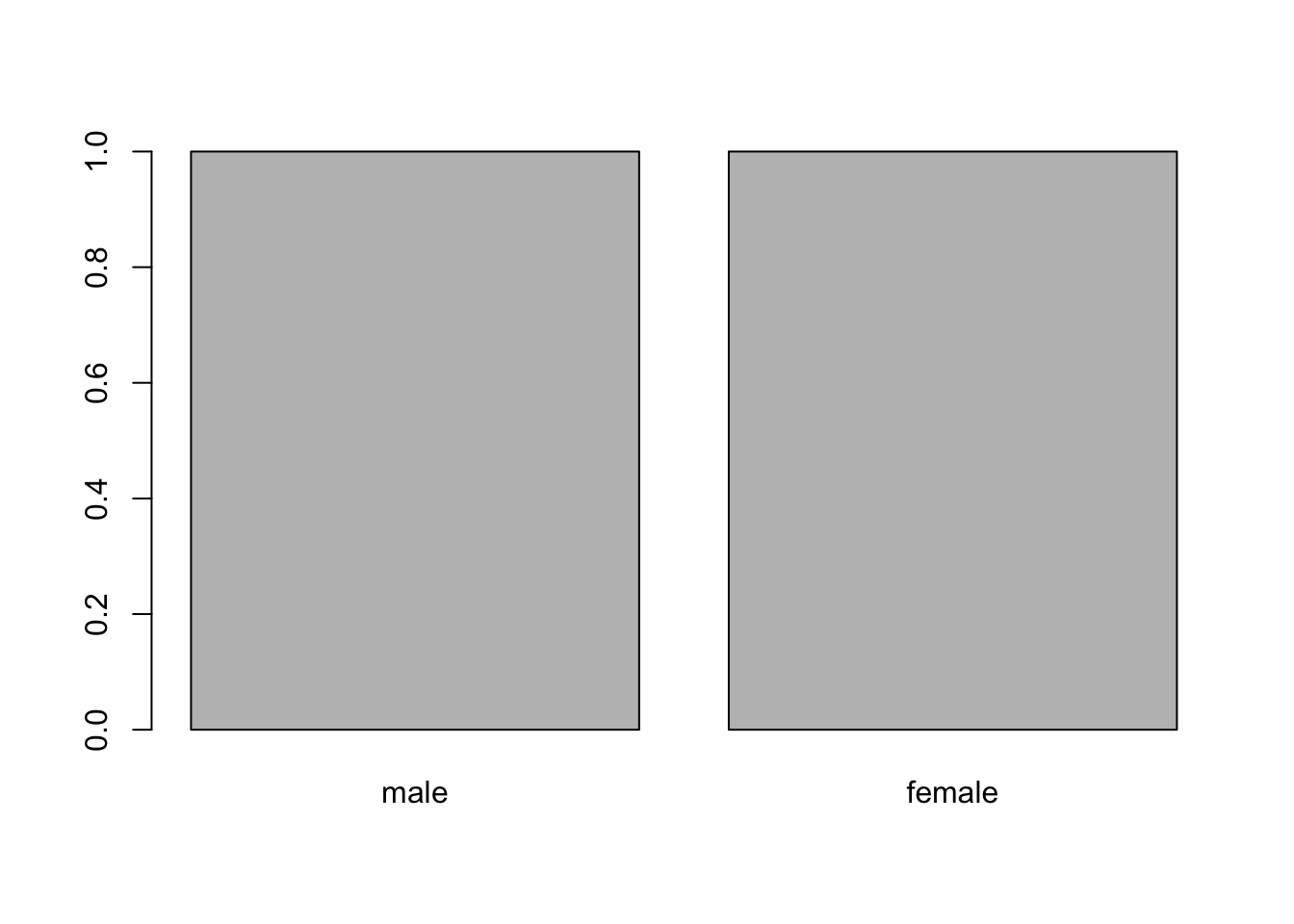
10.7.2 mutate + recode or fct_recode
With many options and functions, the factor command can be initially confusing. An alternative approach that may avoid confusion, is to use the factor command to convert variables to factors, then use either fct_recode or recode to rename the levels explicitly. fct_recode and recode both use arguments that equate new to old level names but differ in the expected name order. Below is an example of each command used to change “0” and “1” into “female” and “male”:
Code
sex = c(0, 1)
sex = factor(sex)
sex = recode(sex, "0" = "female", "1" = "male")
or…
Code
sex = c(0, 1)
sex = factor(sex)
sex = fct_recode(sex, "female" = "0", "male" = "1")
The factor command is often shorter than the other two because existing level names need not be referenced. However, the recode and fct_recode commands can be shorter for changing a subset of level names and are more explicit. Remember that each of these lines of code would have to be placed inside of a mutate command to be included within a data import pipe chain.
Because of the many ways these commands operate, one should always check the data to ensure the desired outcome is achieved. Below, we use each of these commands inside mutate to change the level names of factor variables in the cholesterol data:
Code
tbl <-
    read_csv(file = "data/cholesterol.csv",
             na = c("N/A", "###", "missing"),
             col_types = 'fnnnfnnnnnn') %>%

    mutate(gender = na_if(gender, 999)) %>%

    pivot_longer(cols = weight_i:ldl_f,
                 names_sep = "_",
                 names_to = c(".value", "timepoint")) %>%

    rename(sex = gender) %>%

    mutate_at(vars(sex, timepoint), as.factor) %>%

    mutate(sex = factor(sex, labels = c('male', 'female')),
           group = recode(group, '0' = 'control', '1' = 'statin'),
           timepoint = fct_recode(timepoint, 'initial' = 'i', 'final' = 'f'))

head(tbl)
# A tibble: 6 × 9
name age sex height group timepoint weight hdl ldl
<fct> <dbl> <fct> <dbl> <fct> <fct> <dbl> <dbl> <dbl>
1 William 26 male 69 control initial 172 49 81
2 William 26 male 69 control final 156 48 86
3 Richard 37 male 67 control initial 184 54 95
4 Richard 37 male 67 control final 165 53 93
5 Joseph 45 male 66 control initial 191 49 106
6 Joseph 45 male 66 control final 180 46 112Most tidyverse commands are designed for piping. However, commands like factor, recode, and fct_recode() that take in and return a vector, instead of a tibble or dataframe, do not function as a direct link in the pipe chain. However, we can still use these commands within mutate() to recode variables without breaking the pipe chain.
10.8 Create variables with ifelse()
ifelse() statements iterate over a vector and return one of two values based on the result of a logical test expression. We often use ifelse() to create new variables based on the values of one or more existing variables. The three required arguments for ifelse()are shown below.
test = <test expressions using relational operators>
yes = <value to return when test == TRUE>
no = <value to return when test == FALSE, OR enter another ifelse>
Below we use ifelse() to create a variable, LetterGrade, that equals “pass” when points are at least 7 and “fail” when points are less than 7.
Code
points = 1:10
LetterGrade = ifelse(test = points >= 7,
           yes = "pass",
           no = "fail")
tibble(points,LetterGrade)
# A tibble: 10 × 2
points LetterGrade
<int> <chr>
1 1 fail
2 2 fail
3 3 fail
4 4 fail
5 5 fail
6 6 fail
7 7 pass
8 8 pass
9 9 pass
10 10 pass 10.9 Nested ifelse() Statements
Nested ifelse() statements create variables with more than two values. For three values, the no = argument introduces a new ifelse() statement.The new ifelse() statement can identify two additional values for a total of three, and is “nested” because it lives within the original ifelse() statement. The nesting process is repeated until all the desired levels are created. Below, we use nested ifelse() commands to create letter grades from points and omit the argument names for brevity and readability.
Code
points = 1:10
LetterGrade = ifelse(points <= 6, "F",
                     ifelse(points < 7, "D",
                            ifelse(points < 8,"C",
                                   ifelse(points < 9, "B", "A"))))
tibble(points,LetterGrade)
# A tibble: 10 × 2
points LetterGrade
<int> <chr>
1 1 F
2 2 F
3 3 F
4 4 F
5 5 F
6 6 F
7 7 C
8 8 B
9 9 A
10 10 A 10.10 Create new variables with ifelse and mutate
To create new variables from existing variables we again use mutate. Below we create a total cholesterol column that is a sum of the hdl and ldl columns. We also create a body mass index (bmi) column from height and weight. Lastly, we add a categorical variable that places individuals into groups based on their age.
Notice that we do not extend the pipe chain below to create tc, bmi, and age_c. We add additional arguments to the mutate command that create the desired variables. Lastly, we use relocate to change the order of variables within the tibble. This optional step is purely organizational and does not affect function.
Code
tbl <-
    read_csv(file = "data/cholesterol.csv",
             na = c("N/A", "###", "missing"),
             col_types = 'fnnnfnnnnnn') %>%

    mutate(gender = na_if(gender, 999)) %>%

    pivot_longer(cols = weight_i:ldl_f,
                 names_sep = "_",
                 names_to = c(".value", "timepoint")) %>%

    rename(sex = gender) %>%

    mutate_at(vars(sex, timepoint), as.factor) %>%

    mutate(sex = factor(sex, labels = c('male', 'female')),
           group = recode(group, '0' = 'control', '1' = 'statin'),
           timepoint = fct_recode(timepoint, 'initial' = 'i', 'final' = 'f'),
           tc = hdl + ldl,
           bmi = (weight/(height)^2) * 703,
           age_c = ifelse(test = age < 31,
                          yes = "20 - 30",
                          no = ifelse(test = age < 41,
                                      yes = '31 - 40',
                                      no = '41 - 55')),
           age_c = factor(age_c)) %>%

    # relocate variables within the tibble
    relocate(age_c, .after = age) %>%
    relocate(bmi, .after = weight)

head(tbl)
# A tibble: 6 × 12
name age age_c sex height group timepoint weight bmi hdl ldl tc
<fct> <dbl> <fct> <fct> <dbl> <fct> <fct> <dbl> <dbl> <dbl> <dbl> <dbl>
1 Willi… 26 20 -… male 69 cont… initial 172 25.4 49 81 130
2 Willi… 26 20 -… male 69 cont… final 156 23.0 48 86 134
3 Richa… 37 31 -… male 67 cont… initial 184 28.8 54 95 149
4 Richa… 37 31 -… male 67 cont… final 165 25.8 53 93 146
5 Joseph 45 41 -… male 66 cont… initial 191 30.8 49 106 155
6 Joseph 45 41 -… male 66 cont… final 180 29.0 46 112 158Import Pipe chains rely upon two critical design features:
the command before the pipe operator must output a tibble or dataframe.
the command after the pipe operator must accept a tibble or dataframe.
Tidyverse commands that meet the above criteria have ‘data = …’ as their first argument.
10.11 More Pivoting Challenges
Sometimes data are produced without the foresight of pivoting. Variable names may not lend themselves to easy separations because they do not use a handy separator, like “\_”. Below are two pivoting examples involving problematic column names.
10.11.1 Special character separators (escaping)
Below, we import the cholesterol data used earlier, but from a file that uses “.” instead of “\_” in variable names. Periods are a poor choice because they are special characters with other meanings in R. However, we can use escape characters, two backslashes, to make R interpret the period as text.
Code
read_csv("data/cholesterol_dot.csv") %>% head(2)# A tibble: 2 × 11
name age sex height group weight.i hdl.i ldl.i weight.f hdl.f ldl.f
<chr> <dbl> <dbl> <dbl> <dbl> <dbl> <dbl> <dbl> <dbl> <dbl> <dbl>
1 William 26 0 69 0 172 49 81 156 48 86
2 Richard 37 0 67 0 184 54 95 165 53 93Code
tbl <-
    read_csv("data/cholesterol_dot.csv") %>%

    pivot_longer(cols = weight.i:ldl.f,
                 names_sep = "\\.",
                 names_to = c(".value", "timepoint"))

head(tbl, 2)
# A tibble: 2 × 9
name age sex height group timepoint weight hdl ldl
<chr> <dbl> <dbl> <dbl> <dbl> <chr> <dbl> <dbl> <dbl>
1 William 26 0 69 0 i 172 49 81
2 William 26 0 69 0 f 156 48 8610.11.2 Pivoting with no separator
10.11.2.1 Using character indexes
In the following two examples, we use a version of the data that has no name separator. Variable names are simply appended with a letter, i or f, that codes for initial and final time points. Fortunately, the names_sep = () argument can break apart variable names based on a character index value. In this case, we can use -1 to break off the last character of each variable name.
Code
read_csv("data/cholesterol_none.csv") %>% head(2)# A tibble: 2 × 11
name age sex height group weighti hdli ldli weightf hdlf ldlf
<chr> <dbl> <dbl> <dbl> <dbl> <dbl> <dbl> <dbl> <dbl> <dbl> <dbl>
1 William 26 0 69 0 172 49 81 156 48 86
2 Richard 37 0 67 0 184 54 95 165 53 93Code
tbl <-
    read_csv("data/cholesterol_none.csv") %>%
    pivot_longer(cols = weighti:ldlf,
                 names_sep = -1,
                 names_to = c(".value", "timepoint"))

head(tbl, 2)
# A tibble: 2 × 9
name age sex height group timepoint weight hdl ldl
<chr> <dbl> <dbl> <dbl> <dbl> <chr> <dbl> <dbl> <dbl>
1 William 26 0 69 0 i 172 49 81
2 William 26 0 69 0 f 156 48 8610.11.2.2 Renaming variables
In this example, the variable names use no separator and instead of appending with single characters, the words initial and final are appended to the variable names. This was another poor choice because there is no easy way to separate the parts of these variable names. One solution is to create new names in R that use an underscore. After renaming, we can pivot using the names_sep = "_" and names_to arguments.
Code
read_csv("data/cholesterol_rename.csv") %>% head(2)# A tibble: 2 × 11
name age sex height group weightinitial hdlinitial ldlinitial weightfinal
<chr> <dbl> <dbl> <dbl> <dbl> <dbl> <dbl> <dbl> <dbl>
1 Will… 26 0 69 0 172 49 81 156
2 Rich… 37 0 67 0 184 54 95 165
# ℹ 2 more variables: hdlfinal <dbl>, ldlfinal <dbl>Code
tbl <-
    read_csv("data/cholesterol_rename.csv") %>%
    rename(weight_initial = weightinitial,
           hdl_initial = hdlinitial,
           ldl_initial = ldlinitial,
           weight_final = weightfinal,
           hdl_final = hdlfinal,
           ldl_final = ldlfinal) %>%
    pivot_longer(cols = weight_initial:ldl_final,
                 names_sep = "_",
                 names_to = c(".value", "timepoint"))

head(tbl, 2)
# A tibble: 2 × 9
name age sex height group timepoint weight hdl ldl
<chr> <dbl> <dbl> <dbl> <dbl> <chr> <dbl> <dbl> <dbl>
1 William 26 0 69 0 initial 172 49 81
2 William 26 0 69 0 final 156 48 8610.12 Pivot long to wide
Occasionally, we may need to pivot data from long to wide format. This is the opposite of pivoting longer. The pivot_wider() function uses similar arguments, called names_from and values_from to accomplish the task. Below, we use the pivot_wider() function to pivot the data from the previous example back to its original form.
Code
tbl_wide <-
    tbl %>%
    pivot_wider(names_from = timepoint,
                values_from = c(weight, hdl, ldl))

tbl_wide %>% head(2)
# A tibble: 2 × 11
name age sex height group weight_initial weight_final hdl_initial
<chr> <dbl> <dbl> <dbl> <dbl> <dbl> <dbl> <dbl>
1 William 26 0 69 0 172 156 49
2 Richard 37 0 67 0 184 165 54
# ℹ 3 more variables: hdl_final <dbl>, ldl_initial <dbl>, ldl_final <dbl>For example, as of July 2, 2024, the t.test() function requires wide data to perform a paired t-test. While this new constraint be temporary and inadvertent, we can use the pivot_wider() function to solve the problem. Below we perform a paired t-test using wide-formatted data.
Code
t.test(x = tbl_wide$weight_initial,
       y = tbl_wide$weight_final,
       paired = TRUE)
    Paired t-test

data:  tbl_wide$weight_initial and tbl_wide$weight_final
t = 18.844, df = 39, p-value < 2.2e-16
alternative hypothesis: true mean difference is not equal to 0
95 percent confidence interval:
 11.20293 13.89707
sample estimates:
mean difference
          12.55
The statistical details of a t-test are outside the scope of this tutorial.