11  Explore Data

Exploratory data analysis (EDA) is learning about a dataset without focusing on preconceived expectations or hypotheses. EDA can reveal unexpected insights, and influence how data are subsequently analyzed. While every data situation is unique, a basic EDA should explore the completeness of the data (AKA missingness), univariate distributions for categorical and quantitative variables, outliers and erroneous or impossible values, and correlations between variables. Simple plots like histograms and bar graphs are created to explore distributions, while tables with measures of center, variation, and frequency are created to explore variables numerically. In this section we start with data that are already wrangled and ready for analysis. However, data wrangling and exploratory data analysis are often intermixed, as data wrangling enables exploratory data analysis, and exploratory data analysis can reveal additional problems with the data.

11.1 Characterize Missing Values

Knowing which variables and observations have missing values can be important for an analysis. At a minimum we should know how many missing values exist and if the missing values are randomly distributed or concentrated at certain timepoints, groups, or other conditions. Below we demonstrate a few simple methods for characterizing missing values using a tibble (tbl) produced in the previous lesson.

Code

# How many missing values exist?
tbl %>% is.na %>% sum

[1] 36

Code

# How many rows have missing values?
tbl %>%
    filter(!complete.cases(tbl)) %>%
    nrow()

[1] 19

Code

# Which variables have missing values?
summary(tbl)

       name         age            age_c        sex         height     
 William : 2   Min.   :21.00   20 - 30:18   male  :36   Min.   :54.00  
 Richard : 2   1st Qu.:32.50   31 - 40:22   female:38   1st Qu.:61.75  
 Joseph  : 2   Median :40.50   41 - 55:40   NA's  : 6   Median :65.00  
 Daniel  : 2   Mean   :39.62                            Mean   :64.65  
 Jennifer: 2   3rd Qu.:47.25                            3rd Qu.:67.00  
 Barbara : 2   Max.   :55.00                            Max.   :74.00  
 (Other) :68                                                           
     group      timepoint      weight           bmi             hdl       
 control:40   initial:40   Min.   :156.0   Min.   :20.03   Min.   :44.00  
 statin :40   final  :40   1st Qu.:177.0   1st Qu.:27.68   1st Qu.:50.00  
                           Median :187.0   Median :31.37   Median :54.00  
                           Mean   :185.7   Mean   :31.88   Mean   :53.69  
                           3rd Qu.:194.0   3rd Qu.:35.28   3rd Qu.:56.50  
                           Max.   :214.0   Max.   :49.18   Max.   :64.00  
                           NA's   :6       NA's   :6       NA's   :5      
      ldl               tc       
 Min.   : 47.00   Min.   :104.0  
 1st Qu.: 82.00   1st Qu.:137.0  
 Median : 93.50   Median :148.0  
 Mean   : 94.32   Mean   :148.2  
 3rd Qu.:107.50   3rd Qu.:162.0  
 Max.   :140.00   Max.   :190.0  
 NA's   :4        NA's   :9      

Code

# Are the total cholesterol missing values balanced across timepoints?
tbl %>%
    group_by(timepoint) %>%
    filter(is.na(tc)) %>%
    summarize("Total Cholesterol NA's" = n())

# A tibble: 2 × 2
  timepoint `Total Cholesterol NA's`
  <fct>                        <int>
1 initial                          4
2 final                            5

11.2 Descriptive Statistics

11.2.1 Base R Commands

Base R uses intuitively named descriptive statistics commands that work with tibbles and vectors. Often the command is as simple as one word with a data object passed into the command.

Code

# Base R commands with tibbles or dataframes
mean(tbl$height)
min(81, 57, 66, 94, 79, 44, 19, 100, 64, 20)
max(tbl$height)
range(81, 57, 66, 94, 79, 44, 19, 100, 64, 20)
sd(tbl$age)

# Base R commands with vectors
mean(0:100)
min(0:100)
max(0:100)
range(0:100)
sd(0:100)

11.2.2 The summary command

Like many commands in R, summary() uses different methods for different object types. As shown below, summary() will produce different outputs for tibbles, factor vectors, and numeric vectors.

Code

summary(tbl$age)

   Min. 1st Qu.  Median    Mean 3rd Qu.    Max. 
  21.00   32.50   40.50   39.62   47.25   55.00 

Code

summary(tbl$sex)

  male female   NA's 
    36     38      6 

Code

summary(tbl)

       name         age            age_c        sex         height     
 William : 2   Min.   :21.00   20 - 30:18   male  :36   Min.   :54.00  
 Richard : 2   1st Qu.:32.50   31 - 40:22   female:38   1st Qu.:61.75  
 Joseph  : 2   Median :40.50   41 - 55:40   NA's  : 6   Median :65.00  
 Daniel  : 2   Mean   :39.62                            Mean   :64.65  
 Jennifer: 2   3rd Qu.:47.25                            3rd Qu.:67.00  
 Barbara : 2   Max.   :55.00                            Max.   :74.00  
 (Other) :68                                                           
     group      timepoint      weight           bmi             hdl       
 control:40   initial:40   Min.   :156.0   Min.   :20.03   Min.   :44.00  
 statin :40   final  :40   1st Qu.:177.0   1st Qu.:27.68   1st Qu.:50.00  
                           Median :187.0   Median :31.37   Median :54.00  
                           Mean   :185.7   Mean   :31.88   Mean   :53.69  
                           3rd Qu.:194.0   3rd Qu.:35.28   3rd Qu.:56.50  
                           Max.   :214.0   Max.   :49.18   Max.   :64.00  
                           NA's   :6       NA's   :6       NA's   :5      
      ldl               tc       
 Min.   : 47.00   Min.   :104.0  
 1st Qu.: 82.00   1st Qu.:137.0  
 Median : 93.50   Median :148.0  
 Mean   : 94.32   Mean   :148.2  
 3rd Qu.:107.50   3rd Qu.:162.0  
 Max.   :140.00   Max.   :190.0  
 NA's   :4        NA's   :9      

NOTE Summary Methods

When we load packages such as tidyverse, those packages often add additional methods to commands like summary(). Presently, base R has 32 methods available for summary(). Loading tidyverse adds another 15 methods for a total of 47. A powerful R feature is that we do not have to choose from this list explicitly. R recognizes the type of object and applies the appropriate method.

11.2.3 R looping functions

Base R includes a collection of “apply” functions that are designed to apply a function over the elements of a list, tibble or vector. The most common are apply(), sapply() and lapply().

11.2.3.1 apply()

apply() runs a command over either the rows (MARGIN = 1) or columns (MARGIN = 2) of a tibble, dataframe, or matrix (not covered). Below we use apply() to calculate the mean of every numeric variable in tbl. The first argument identifies a subset of tbl, where we have used select_if() to choose only the variables that are numeric.

Code

apply(X = select_if(tbl, is.numeric),
      MARGIN = 2,
      FUN = mean)

   age height weight    bmi    hdl    ldl     tc 
39.625 64.650     NA     NA     NA     NA     NA 

11.2.3.2 lapply()

lapply() functions like apply() but always returns output as a list.

Code

tbl %>% select_if(is.numeric) %>% lapply(mean)

$age
[1] 39.625

$height
[1] 64.65

$weight
[1] NA

$bmi
[1] NA

$hdl
[1] NA

$ldl
[1] NA

$tc
[1] NA

11.2.3.3 sapply()

sapply() functions like apply(), but returns output using the most simple base R data structure possible, which could be a list, dataframe, or vector depending on the scenario.

Code

tbl %>% select_if(is.numeric) %>% sapply(mean)

   age height weight    bmi    hdl    ldl     tc 
39.625 64.650     NA     NA     NA     NA     NA 

11.2.4 Ignoring NA’s

R commands don’t ignore NA by default, as demonstrated below.

Code

mean(tbl$hdl)

[1] NA

Code

tbl %>%
    ggplot(aes(x = sex, y = hdl)) +
    geom_bar(stat = 'summary',
             fun = mean)

Warning: Removed 5 rows containing non-finite outside the scale range
(`stat_summary()`).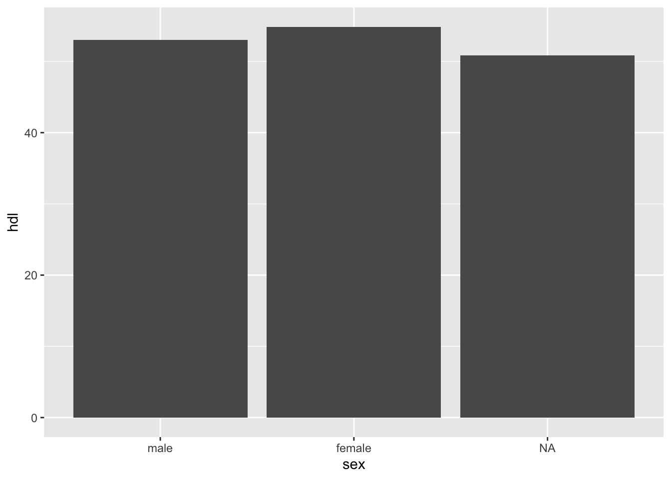

11.2.4.1 na.rm = TRUE

The na.rm = TRUE tells R to remove (ignore) NAs

Code

mean(tbl$hdl, na.rm =TRUE)

[1] 53.69333

11.2.4.2 drop_na

The drop_na commad will drop all rows with any missing values (default) or will drop rows with missing values for specific columns.

Code

# drop all rows with any missing values
tbl %>%
    drop_na %>%
    summary

       name         age            age_c        sex         height     
 William : 2   Min.   :21.00   20 - 30:16   male  :31   Min.   :54.00  
 Richard : 2   1st Qu.:30.00   31 - 40:14   female:30   1st Qu.:62.00  
 Joseph  : 2   Median :41.00   41 - 55:31               Median :65.00  
 Jennifer: 2   Mean   :39.69                            Mean   :65.08  
 Jessica : 2   3rd Qu.:47.00                            3rd Qu.:67.00  
 Emily   : 2   Max.   :55.00                            Max.   :74.00  
 (Other) :49                                                           
     group      timepoint      weight           bmi             hdl       
 control:29   initial:30   Min.   :156.0   Min.   :20.03   Min.   :44.00  
 statin :32   final  :31   1st Qu.:177.0   1st Qu.:27.32   1st Qu.:50.00  
                           Median :185.0   Median :30.50   Median :54.00  
                           Mean   :185.2   Mean   :31.38   Mean   :53.84  
                           3rd Qu.:194.0   3rd Qu.:34.76   3rd Qu.:57.00  
                           Max.   :205.0   Max.   :49.18   Max.   :64.00  
                                                                          
      ldl               tc       
 Min.   : 47.00   Min.   :104.0  
 1st Qu.: 81.00   1st Qu.:137.0  
 Median : 93.00   Median :146.0  
 Mean   : 93.48   Mean   :147.3  
 3rd Qu.:109.00   3rd Qu.:161.0  
 Max.   :140.00   Max.   :190.0  
                                 

Code

# drop rows with missing values in specific columns
tbl %>%
    drop_na(sex, hdl) %>%
    ggplot(aes(x = sex, y = hdl)) +
    geom_bar(stat = 'summary',
             fun = mean)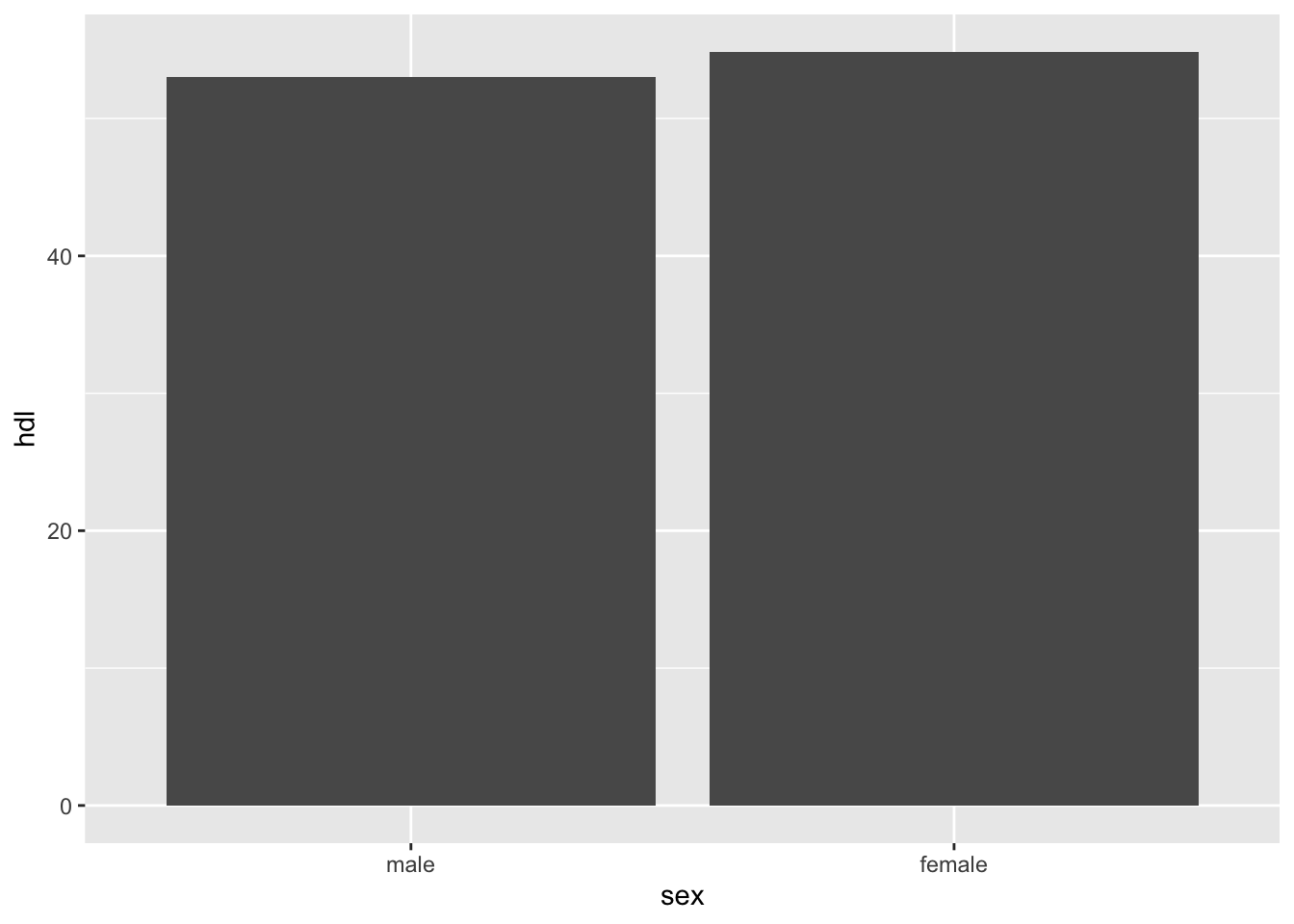

11.3 Distributions & Bivariate Relationships

Distributions present the values of a variable and the frequency each value is observed. Exploring distributions tell us qualitative information about center, variation, shape, and outliers and identify strengths and limitations in the data, such as normal distributions (a strength) and imbalanced experimental designs (a weakness). In the exploratory data analysis phase, we generally want to explore many possible relationships and are not yet creating polished graphs for publication.

11.3.1 GGally::ggpairs

The tidyverse-aligned command ggpairs() from the GGally package creates plot mosaics that are helpful for exploring many distributions and relationships with just a few lines of code.

11.3.1.1 Categorical Distributions and Bivariate Relationships

Code

tbl %>% 
    filter(timepoint == "initial") %>%
    select(age_c, sex, group) %>%
    drop_na() %>%
    ggpairs(showStrips = TRUE)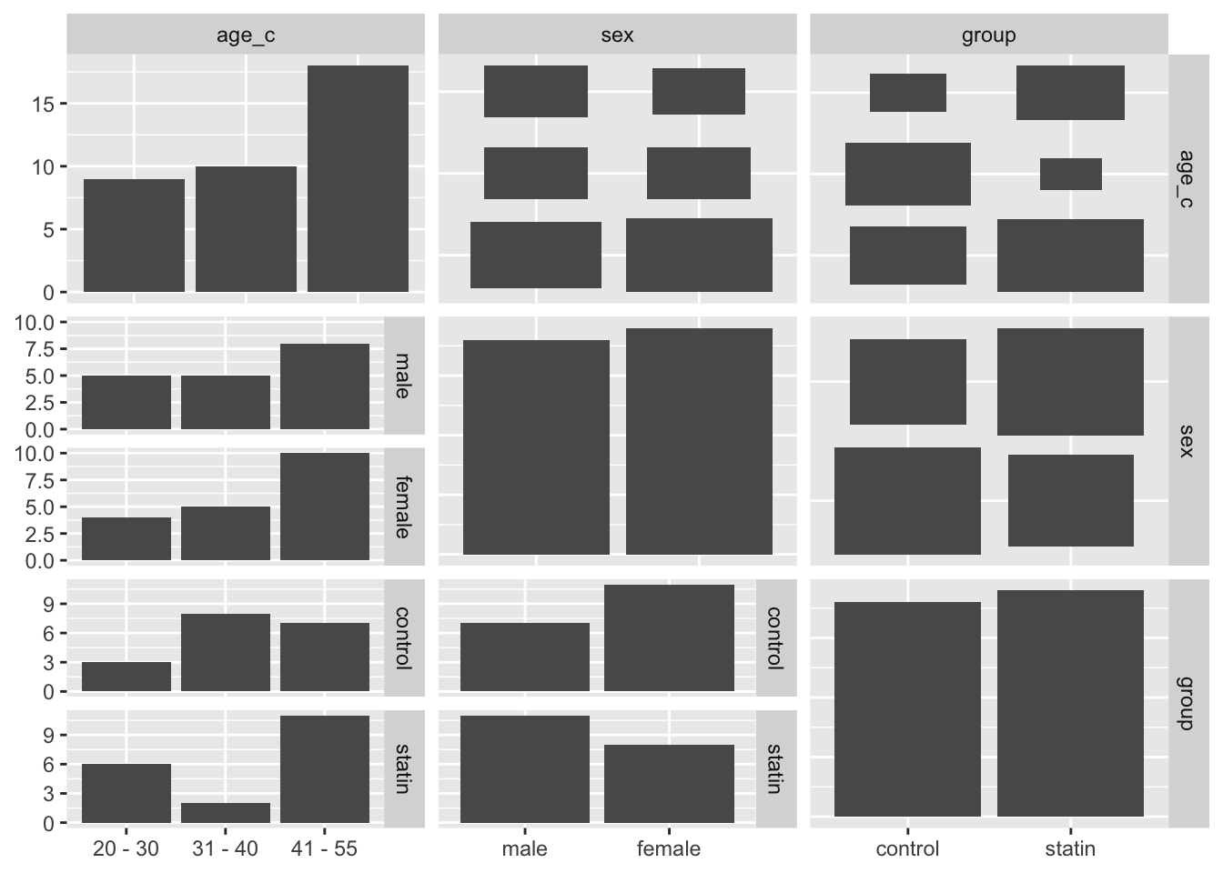

11.3.1.2 Quantitative distributions & Bivariate Relationships

Code

tbl %>%
    filter(timepoint == 'initial') %>% 
    select(where(is.numeric)) %>%
    drop_na() %>%
    ggpairs()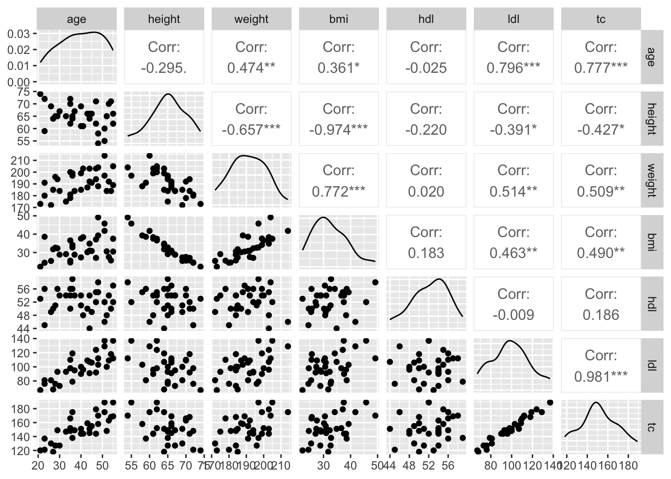

11.3.1.3 Specific Quantitative distributions & Bivariate Relationships, Colored by Factor

Code

pm <- 
    tbl %>%
    filter(timepoint == 'initial') %>%
    drop_na() %>%
    ggpairs(aes(color = sex), columns = c('age', 'bmi', 'hdl', 'ldl', 'tc'))
pm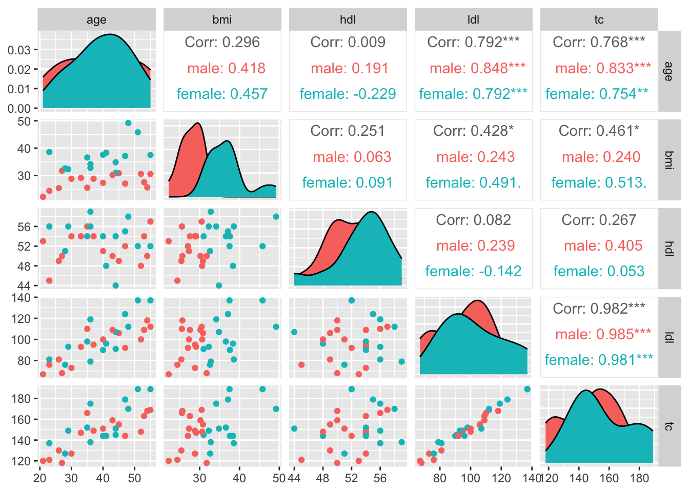

11.3.1.4 Isolate and Customize Plots

With the plot mosaic assigned to an object name (“pm” above), we can use base R brackets to isolate and customize a plot with additional ggplot layers. Below, we isolate and enhance the subplot located in row 5, column 1. A detailed coverage of ggplot layers is provided in lesson 12.

Code

pm[5,1] + 
    labs(y = "total cholesterol (ng/dl)") + 
    geom_smooth(method = 'lm', se = F) +
    theme_bw()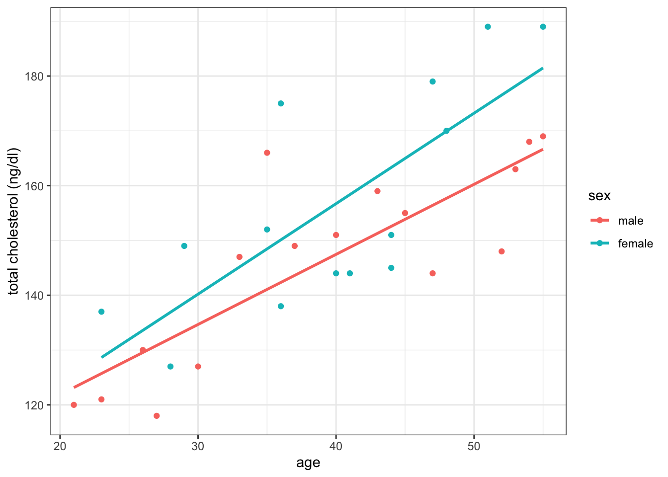

11.4 Frequency tables

Frequency tables show the counts at each level of a categorical variable. When a frequency table includes a second categorical variable, it is called a two-way table. The base R table() command provides this information, as demonstrated below.

Code

table(tbl$sex, tbl$group)

        
         control statin
  male        14     22
  female      22     16

Code

# Add HTML formatting with commands from knitr::kable and kableExtra::kable_classic

table(tbl$sex, tbl$group) %>%
    kable() %>% 
    kable_classic(full_width = F)

	control	statin
male	14	22
female	22	16

11.5 Frequency Tables with Janitor Package

With multiple categorical variables, we often wish to know conditional percentages in addition to observation counts. The Janitor package provides the tabyl() (spelled with a ‘y’) command for creating frequency tables with conditional percentages, and has the added benefit of being tidyverse aligned. However, janitor is not imported with tidyverse and must be loaded with a separate library command, or added to the package list in p_load().

Code

library(janitor) 

# Load and preview the starwars data
data(starwars, package = 'dplyr')
glimpse(starwars)

Rows: 87
Columns: 14
$ name       <chr> "Luke Skywalker", "C-3PO", "R2-D2", "Darth Vader", "Leia Or…
$ height     <int> 172, 167, 96, 202, 150, 178, 165, 97, 183, 182, 188, 180, 2…
$ mass       <dbl> 77.0, 75.0, 32.0, 136.0, 49.0, 120.0, 75.0, 32.0, 84.0, 77.…
$ hair_color <chr> "blond", NA, NA, "none", "brown", "brown, grey", "brown", N…
$ skin_color <chr> "fair", "gold", "white, blue", "white", "light", "light", "…
$ eye_color  <chr> "blue", "yellow", "red", "yellow", "brown", "blue", "blue",…
$ birth_year <dbl> 19.0, 112.0, 33.0, 41.9, 19.0, 52.0, 47.0, NA, 24.0, 57.0, …
$ sex        <chr> "male", "none", "none", "male", "female", "male", "female",…
$ gender     <chr> "masculine", "masculine", "masculine", "masculine", "femini…
$ homeworld  <chr> "Tatooine", "Tatooine", "Naboo", "Tatooine", "Alderaan", "T…
$ species    <chr> "Human", "Droid", "Droid", "Human", "Human", "Human", "Huma…
$ films      <list> <"A New Hope", "The Empire Strikes Back", "Return of the J…
$ vehicles   <list> <"Snowspeeder", "Imperial Speeder Bike">, <>, <>, <>, "Imp…
$ starships  <list> <"X-wing", "Imperial shuttle">, <>, <>, "TIE Advanced x1",…

Code

# Convert character variables into factors using mutate_at
starwars %<>% 
    mutate_at(vars(hair_color, skin_color, eye_color, sex, gender, homeworld, species), 
              as.factor)

# A simple one-way frequency table using tabyl with HTML formatting provided by kable() %>% kable_classic(full_width = F)
starwars %>% 
    tabyl(eye_color) %>% 
    adorn_rounding(2) %>%
    kable() %>% kable_classic(full_width = F)

eye_color	n	percent
black	10	0.11
blue	19	0.22
blue-gray	1	0.01
brown	21	0.24
dark	1	0.01
gold	1	0.01
green, yellow	1	0.01
hazel	3	0.03
orange	8	0.09
pink	1	0.01
red	5	0.06
red, blue	1	0.01
unknown	3	0.03
white	1	0.01
yellow	11	0.13

Code

# A two-way table for eye color and gender for non-droids using tabyl
starwars %>%
    filter(species != 'Droid') %>%
    tabyl(gender, eye_color) %>% 
    kable() %>% kable_classic(full_width = F)

gender	black	blue	blue-gray	brown	dark	gold	green, yellow	hazel	orange	pink	red	red, blue	unknown	white	yellow
feminine	2	6	0	4	0	0	0	2	0	0	0	0	1	0	1
masculine	7	12	1	15	1	1	1	1	8	1	2	0	2	0	9

11.5.1 “adorn” frequency table with details

After the initial table setup using tabyl(), we “adorn” the table with additional features linked together in a pipe chain. Lastly, because the output is still a tibble, we can pipe into the kable() and kable_classic commands to create an aesthetically pleasing table ready for presentation or publication.

Code

starwars %>%
    filter(species == 'Human') %>%
    tabyl(gender, eye_color) %>%

    # add totals, conditional percents, rounding
    adorn_totals(c("row", "col")) %>%
    adorn_percentages("row") %>% 
    adorn_pct_formatting(rounding = "half up", digits = 0) %>%
    
    # add sample sizes in parentheses
    adorn_ns() %>% 
    
    # add a title
    adorn_title("combined", 
                row_name = "Gender", 
                col_name = "Eye Color") %>%
    
    # add nice aesthetics
    kable %>% kable_classic(full_width = FALSE)

Gender/Eye Color	black	blue	blue-gray	brown	dark	gold	green, yellow	hazel	orange	pink	red	red, blue	unknown	white	yellow	Total
feminine	0% (0)	33% (3)	0% (0)	44% (4)	0% (0)	0% (0)	0% (0)	11% (1)	0% (0)	0% (0)	0% (0)	0% (0)	11% (1)	0% (0)	0% (0)	100% (9)
masculine	0% (0)	35% (9)	4% (1)	46% (12)	4% (1)	0% (0)	0% (0)	4% (1)	0% (0)	0% (0)	0% (0)	0% (0)	0% (0)	0% (0)	8% (2)	100% (26)
Total	0% (0)	34% (12)	3% (1)	46% (16)	3% (1)	0% (0)	0% (0)	6% (2)	0% (0)	0% (0)	0% (0)	0% (0)	3% (1)	0% (0)	6% (2)	100% (35)

11.6 Pivot tables with group_by() & summarize()

Pivot tables present descriptive information about data grouped at the levels of one or more categorical variables. This is a useful approach when we wish to compare characteristics between males and females, or across ethnicity, age groups, treatment groups, etc.

The tidyverse commands group_by() and summarize() work together to create new tibbles, “pivot tables”, with summary statistics, grouped by one or more factor variables. When we produce these summary tibbles for reports and presentations, we often break the naming rules by including spaces and enclosing the name in quotes as shown below. Lastly, we use commands from the knitr and kableExtra packages to format our tibble with publication-ready aesthetics.

Pivot table with one grouping variable:

Code

tbl %>% 
    
    drop_na(sex) %>%
    
    group_by(sex) %>% 
    
    summarize(Count = n(),
              'Age Mean' = mean(age) %>% round,  
              'Age min' = min(age),
              'Age max'= max(age),
              'Age SD' = sd(age) %>% round) %>%
    
    kable() %>% # kable is from knitr
    
    kable_classic(full_width = F) # kable_classic is from kableExtra

sex	Count	Age Mean	Age min	Age max	Age SD
male	36	39	21	55	11
female	38	39	23	55	9

Pivot table with two grouping variables and nice formatting:

Code

tbl %>%
    
    drop_na(sex) %>%
    
    group_by(sex, group) %>%
    
    summarize(Count = n(),
              'Age Mean' = mean(age) %>% round,  
              'Age min' = min(age),
              'Age max'= max(age),
              'Age SD' = sd(age) %>% round) %>%
    
    kable() %>% # kable is from knitr
    
    kable_classic(full_width = F) # kable_classic is from kableExtra

`summarise()` has grouped output by 'sex'. You can override using the `.groups`
argument.

sex	group	Count	Age Mean	Age min	Age max	Age SD
male	control	14	39	26	54	9
male	statin	22	39	21	55	12
female	control	22	38	23	51	8
female	statin	16	41	23	55	11